Leachate Measurement

Over time, leachate treatment and disposal can represent one of the largest operational costs incurred by a landfill. Even though leachate treatment costs per gallon are often measure in fractions of a cent, the potentially large quantities of leachate generated at even a moderately sized landfill can tally up to a significant monthly fee.

Leachate production by its very nature is unpredictable and is dependent on such multiple variables as climate, season, type of cover, or thickness of waste. Therefore, leachate production cannot be projected or estimated; it has to be directly measured on a continuous basis. Traditional methods of flow measurement can be utilized by landfills, but a relatively new type of measuring mechanism—one based on ultrasonic waves—has the potential for greater accuracy and increased operational flexibility.

Production and Prediction
What exactly is leachate? Leachate is produced by the percolation of precipitation (both rainfall and snowmelt) through the landfill’s daily, intermediate, or final cover. As the water passes vertically downward through the waste mass, it comes into contact with the waste, picking up chemical contaminants and biological impurities as it goes. The question is, then: How much leachate can a landfill expect to produce during its operational lifetime and post-closure care period? The answer of course is: “It depends.”

The primary factor affecting leachate production is the current state of the cover overlying the landfill’s waste. It is a truism that the best leachate management system is a good cap and cover. This cover can consist of only 6 inches of soil cover (daily cover), 12 inches of soil (intermediate cover), or a complete, compacted clay cap with geomembrane overlain by cover soil which has been fully vegetated (final cover). Theoretically, a complete final cap and cover system should completely shed precipitation and prevent any water from entering the deposited waste. In reality, there is always some percolation (though drastically reduced when compared with other covers) even when a final cap and cover is in place.

At the other extreme is the simple daily cover, which usually is placed over the thinner layers of waste that occur during the early stages of disposal operations. This means the greatest amount of percolation usually occurs when there is the least amount of travel distance to the collection layer at the bottom of the landfill—which is the condition for maximum leachate production. Between the extremes of final and daily cover conditions, leachate production can vary widely during the operational lifetime of the landfill.

As the precipitation percolates down through the current cover, it passes through the underlying waste. Municipal solid waste is very heterogeneous in terms of its physical components and in terms of its chemical characteristics. A discarded sofa can lie next to a bag of grass clippings, under a pallet of newspapers, and over a pile of crushed aluminum cans. It is impossible to analyze in detail and predict with minute accuracy the flow path taken by the leachate or the characteristics of the waste with which it comes into contact. However, general predictions of leachate production can be made to provide a reasonably accurate projection of what should be typical of average leachate production through out the landfill’s existence.

For planning purposes, it is assumed that waste (once its variability has been averaged out across the landfill) has certain typical values for permeability. On average, waste has a percolation rate of approximately 1 x 10^-3 cubic centimeters per second. This again is an average for a waste mass that may include significant channels and rifts where streams of leachate can flow freely and layers of old soil cover, compacted to the point of effectively blocking leachate migration and causing leachate mounding, to occur within the waste mass. The assumed percolation rate through the waste is equivalent to almost 0.0004 inches per second, or 2.9 feet per day. So for a typical landfill with an average waste thickness of 200 feet, leachate should not even appear at the bottom of the landfill for almost 70 days. However, precipitation occurs at more or less regular intervals through the disposal process. If a significant rainfall occurs soon after a disposal cell receives waste, large amounts of leachate can be produced almost immediately. In dry climates, significant leachate production may never occur.

Furthermore, waste is assumed to have an average field capacity of almost 30% by volume. Field capacity is defined as the amount of moisture retained by a “soil” after prolonged gravity drainage from a saturated condition. Depending on the initial moisture content (and assuming that there is no leachate recirculation performed at the landfill), the same 200-foot-thick layer of waste could absorb up to 60 feet (720 inches) of precipitation until it achieves field capacity and longer retains percolating leachate. The eastern (and wetter) portion of the continental United States receives 20 to 40 inches per year. So our landfill example could (theoretically) not see any leachate for 36 to 18 years. Because of the heterogeneous nature of waste described above, this doesn’t happen. But it is a useful illustration of how difficult it is to accurately predict leachate formation rates.

Collection and Extraction
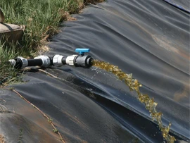
How is leachate removed from a landfill? Once water passes downward through the waste it cannot be allowed to collect and build up on the landfill’s floor. To prevent excessive head build up (defined as more than 12 inches of depth) a system of perforated pipe drains set in mounds of aggregate filter stone and connected by a layer of high-permeability sand is installed on top of the landfill’s liner. The landfill floor is sloped so that leachate flows through the sand layer along the top of the liner until it reaches a perforated collection pipe. The pipe alignment is also given a positive gradient, so the accumulated flows carried by the pipes are directed to central collection points called sumps. The sumps are recessed areas in the landfill floor where leachate is allowed to build up so it can be easily extracted from the landfill.

Extraction is performed by a submersible pump set in the bottom of the sump. The pump discharges through a flexible hose that is housed inside a protective riser pipe and is connected to a force main located outside the landfill perimeter. Leachate flows through the force main(s) until it gets to a storage and/or pretreatment facility. This usually consists of underground or aboveground storage tanks and pretreatment to perform rudimentary cleanup of the leachate (such as BOD reduction) before it is finally disposed of. Disposal usually involves direct discharge to a nearby sanitary sewer or hauling via tanker truck to the wastewater treatment plant. It is often leachate disposal that represents the landfill’s single most expensive operation cost. For this reason alone, it is imperative that leachate flows are measured as accurately and quickly as possible. These measurements are performed by flow meters installed along the force main are at the final discharge point.

Traditional Flow Meters
A flow meter is a device that measures the volume flow of fluids (liquids or gases—or leachate) flowing though a pipe, either directly by measuring volume displacement over a period of time, or indirectly by measuring the velocity of the flow.

Mass flow meters measure actual masses of liquids by means of mechanical displacement. This is usually accomplished with a piston or rotary piston assembly. As the piston rotates in its chamber, a fixed amount of liquid enters and then leaves the chamber. The number of piston cycles per duration determines the flow rate with the number of cycles being measured by an odometer, or gear mechanism. In addition to piston displacement meters, there are paddle-wheel and radial turbine meters. In both cases, flow velocity is measured by the rate of spin imparted to the wheel or turbine by the moving liquid.

Certain types of meters measure flow indirectly by means of pressure differentials. A Venturi meter constricts flow by reducing the diameter of the pipe as it enters the meter. Flow rate can be determined by the pressure change across the meter. Orifice plate meters, Pitot tubes, and Dall tubes work on a similar principle.

Optical flow meters utilize a pair of laser and matching photo-detectors. Both lasers beam a steady stream of light into the liquid. As a particle or air bubble in the flow stream passes through one laser, it reflects the light back to the photo-detector. As the same particle passes through the second laser another reflection and detection occurs. The time difference between the two events over the fixed distance between the two lasers determines the fluid’s flow velocity, and with it the flow rate.

Similar to optical flow meters, thermal flow meters utilize a heating element flanked by a pair of heat sensors working in tandem. As the heat source increases the temperature of the gas flowing past it, knowledge of the fluid’s specific heat, thermal conductivity, and density allow for a determination of flow velocity based on the temperature difference between the upstream and downstream heat sensors.

Coriolis flow meters utilize the Coriolis effect, causing laterally vibrating pipes to distort and bend rhythmically to directly measure fluid flows. Also called a mass flow meter or an inertial flow meter, it measures the amount of mass (not volume) of fluid flowing through a pipe. Given the density of the fluid flowing in the pipe, the mass flow measurement can be used to determine the volumetric flow of the liquid. The meter consists of a pair of thin, parallel, bent tubes that split the fluid flow passing through the pipe. An actuator induces a horizontal vibration in the tubes. This rapid side-to-side movement induces Coriolis effect in the fluid flow. When the mass of the liquid flows through the pipes, the movement of the mass through the vibrating pipes causes the pipes to bend. The asymmetrical bending of the pipes occurs at a frequency and degree of phase shift that is proportional to the mass flow.

Vortex flow meters induce turbulence in the flow by means of a shedder bar placed across the flow path inside the pipe. The resulting turbulence creates vortexes in the fluid stream. The appearance of the vortexes is alternated on either side of the bar at regular interval proportional to the flow rate. A downstream sensor measures the frequency of the vortex shedding by the creation of a small electrical current in the sensor’s piezoelectric crystal, responding to pressure changes in the flow.

In addition to true flow meters there are flow-rate meters. Instead of directly measuring the volume of gas or liquid that enters and leaves its body over fixed time duration, flow-rate meters measure the speed of the fluid flow. By combining the cross-sectional area of the pipe with the measured flow velocity, a flow volume can be calculated.

Not as accurate as true flow meters, flow-rate meters tend to be of simpler design, typically relying on a simple turbine that spins as the fluid flows. Set half in liquid, the blades of the spinning turbine trap and then release discrete volumes of gas flowing into the meter as a geared assembly measures the number of turns made by the blades and, with it, the amount of gas flowing through the meter.

Optisonic Technology
A more recent development in flow meter technology involves the utilization of ultrasonic waves propagated through the fluid and reflected back onto measuring sensors. All ultrasonic flow meters are based on the Doppler effect. It was discovered that a stationary listener receives shorter wavelengths from an approaching source and longer wavelengths from a receding source. Approaching shorter wavelengths sound shriller while receding longer wavelengths have a lower pitch. This frequency shift is measurable and can be used to calculate the flow velocities of fluid in a pipe. In fact, the change in frequency is directly proportional to the flow velocity. More precisely, the velocity being measured is the speed of movement of “discontinuities” in the fluid stream. Given the impurities inherent in leachate, this approach can be a very effective and accurate means of measuring leachate flows. These discontinuities include particles, turbulence waves, or entrapped air bubbles. This makes ultrasonic flow meters useful for measuring the flows of mixed media, especially industrial liquids, such as slurries, fuels, pulps—and leachate from landfills.

The Krohne Corp. produces the Optisonic model line of ultrasonic flow meters that utilize the transit time differential method. The transit time differential method utilizes a pair of ultrasonic waves propagated into the flowing liquid at acute angles to the direction of flow. One of these waves travels in the general direction of the flow and the other travels against the flow. Since it receives that added velocity vector from the flow itself, the wave traveling with the direction of flow can reach the opposite side of the pipe faster than the wave traveling against the flow. In the second case, the flow’s velocity vector is subtracted from the wave velocity since they are traveling in opposite directions.

The two waves are similar to two boats crossing a river on the same diagonal line, one with the flow and the other against the flow. The boat moving with the flow needs much less time to reach the opposite bank. In both cases, the object traveling with the flow moves faster than the object moving against the flow. The system’s sensors continuously measure the transit time for both ultrasonic waves. The difference in the transit time of both waves is directly proportional to the mean flow velocity of the fluid in the pipeline.

Once the flow velocity of the fluid has been determined, the flow rate can be calculated by multiplying the mean flow velocity by the cross-section area of the pipeline. Mean flow velocity is utilized, since the actual flow velocities vary somewhat within the stream. Because of the frictional drag, liquid adjacent to the pipe walls travels somewhat slower than fluid in the center of the pipe.

Measurement of the transit time can also be used to determine the type of liquid flowing through the pipe. This is due to the fact that waves travel at different velocities in media having different densities. The transit time in water is shorter than that of crude oil, assuming a consistent pipe diameter and resultant travel distance for the ultrasonic wave. The flow meters can be calibrated for different pipe diameters and fluid types.

This calibration takes place in the factory prior to shipment. Every flow meter is tested by wet calibration via direct volume comparisons. This method ensures high accuracy for volumetric flow meters. The testing rigs themselves are typically 10 times more accurate that the flow meters being tested. This factor of 10 allows for a large margin of safety against erroneous measurement.

Optisonic Products and Specifications
Krohne’s Optisonic model 6300 is a clamp-on flow meter that can be fitted on the outside of pipes to measure their liquid flow rates. This removes the need for expensive in-flow pipe connections and appurtenances. By utilizing clamp-on flow meters, flow measurements can be taken easily from any point in the pipe network. The Optisonic 6300 also utilizes a “re-greasing” concept that allows for easy handling and rugged manufacture that ensures long-term reliability.

The Optisonic 6300 is actually a hybrid of one or two model Optisonic 6000 clamp-on sensors in combination with one model UFC 300 ultrasonic flow converter. It can be fitted to pipes made from metal, ceramic, asbestos cement, and coated pipes that are internally or externally lined with bonded coatings. It can measure through pipe wall thicknesses of to 200 mm.

Small-scale applications include the measurement of flows in chemical additive feed lines and coolant inside cooling coils. For larger-scale applications, the Optisonic 6300 can be used to measure purified water flows, liquid fuels and other hydrocarbons, and large-pipe-size water and wastewater flows. It has found widespread use in general process control of multiple industrial applications for chemical and petrochemical plants, power-plant cooling water, and district heating water, water distribution systems, oil and gas pipelines, pharmaceuticals, and food processing.

Krohne’s Optisonic model 7060 is a compact gas-flow measuring system that integrates specially designed ultrasonic transducers integrated with a protected cable communication system (including a converter signal processing unit), all manufactured as part of a single meter body. The integrated structure and relatively small size make it suitable for harsh operating conditions. The flow meter will operate accurately, no matter what the low conditions (density, pressure, and temperature) are for the gas being measured. This makes a nearly universal application for all kinds of gas-pipeline flow measurements.

In keeping with its wide range of potential applications, it comes with extensive diagnostic functions (easily accessible through a standard software package). Its operational flexibility allows for bidirectional flow measurement, operations in a wide temperature range, and a high turndown ratio. Its small size takes advantage of all metal miniaturized transducers, which need minimal power consumption (less than 1 watt).

The design of the model 7060 minimizes maintenance requirements while ensuring long-term measurement consistency. The meter body includes special flanges for installation and a section for mounting the transducers. In addition to minimal maintenance, its small size and concealed cabling minimize the chance of physical damage and subsequent repair work. The meter bodies themselves are manufactured from carbon steel or stainless steel and come in several sizes. The specially designed, compatible components are assembled into a single unit that integrates the ultrasonic sensors directly into the meter body.

Prior to delivery, the ultrasonic transducers are optimized to suit the system being measured. This has allowed the model 7060 to be utilized in a wide variety of industrial gas flow applications: chemical and petrochemical, power stations, and compressed air distribution. Accuracy is ensured by highly stable propagation time measurements recorded by the transducers with nanosecond precision.